Classification example: recognize handwritten digits#
This chapter is inspired by the book Hands-On Machine Learning written by Aurélien Géron.
Learning objectives#
Discover how to train a Machine Learning model on bitmap images.
Understand how loss and model performance are evaluated in classification tasks.
Discover several performance metrics and how to choose between them.
Environment setup#
import platform

import numpy as np
import matplotlib.pyplot as plt
import seaborn as sns

import sklearn
from sklearn.datasets import fetch_openml
from sklearn.model_selection import train_test_split, cross_val_score
from sklearn.metrics import (
    ConfusionMatrixDisplay,
    classification_report,
    log_loss,
)
from sklearn.linear_model import SGDClassifier
# Setup plots

# Include matplotlib graphs into the notebook, next to the code
# https://stackoverflow.com/a/43028034/2380880
%matplotlib inline

# Improve plot quality
%config InlineBackend.figure_format = "retina"

# Setup seaborn default theme
# http://seaborn.pydata.org/generated/seaborn.set_theme.html#seaborn.set_theme
sns.set_theme()
# Print environment info
print(f"Python version: {platform.python_version()}")
print(f"NumPy version: {np.__version__}")
print(f"scikit-learn version: {sklearn.__version__}")
Python version: 3.11.1
NumPy version: 1.26.4
scikit-learn version: 1.4.1.post1
Context and data preparation#
The MNIST handwritten digits dataset#
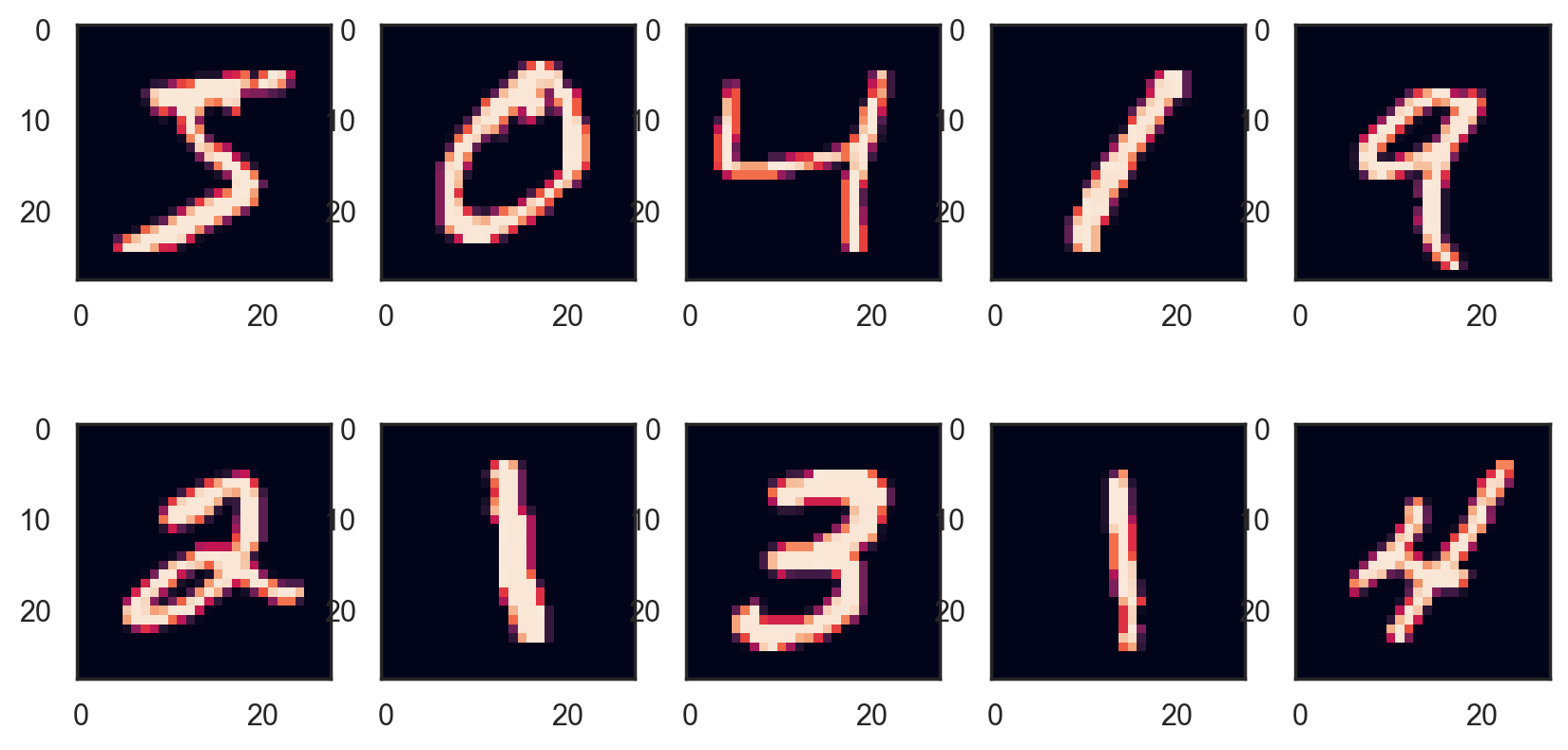
This dataset, a staple of Machine Learning and the “Hello, world!” of computer vision, contains 70,000 bitmap images of digits.
The associated target (expected result) for any image is the digit its represents.
# Load the MNIST digits dataset from sciki-learn
images, targets = fetch_openml(
    "mnist_784", version=1, parser="pandas", as_frame=False, return_X_y=True
)

print(f"Images: {images.shape}. Targets: {targets.shape}")
print(f"First 10 labels: {targets[:10]}")
Images: (70000, 784). Targets: (70000,)
First 10 labels: ['5' '0' '4' '1' '9' '2' '1' '3' '1' '4']
# Show raw data for the first digit image
print(images[0])
[  0   0   0   0   0   0   0   0   0   0   0   0   0   0   0   0   0   0
   0   0   0   0   0   0   0   0   0   0   0   0   0   0   0   0   0   0
   0   0   0   0   0   0   0   0   0   0   0   0   0   0   0   0   0   0
   0   0   0   0   0   0   0   0   0   0   0   0   0   0   0   0   0   0
   0   0   0   0   0   0   0   0   0   0   0   0   0   0   0   0   0   0
   0   0   0   0   0   0   0   0   0   0   0   0   0   0   0   0   0   0
   0   0   0   0   0   0   0   0   0   0   0   0   0   0   0   0   0   0
   0   0   0   0   0   0   0   0   0   0   0   0   0   0   0   0   0   0
   0   0   0   0   0   0   0   0   3  18  18  18 126 136 175  26 166 255
 247 127   0   0   0   0   0   0   0   0   0   0   0   0  30  36  94 154
 170 253 253 253 253 253 225 172 253 242 195  64   0   0   0   0   0   0
   0   0   0   0   0  49 238 253 253 253 253 253 253 253 253 251  93  82
  82  56  39   0   0   0   0   0   0   0   0   0   0   0   0  18 219 253
 253 253 253 253 198 182 247 241   0   0   0   0   0   0   0   0   0   0
   0   0   0   0   0   0   0   0  80 156 107 253 253 205  11   0  43 154
   0   0   0   0   0   0   0   0   0   0   0   0   0   0   0   0   0   0
   0  14   1 154 253  90   0   0   0   0   0   0   0   0   0   0   0   0
   0   0   0   0   0   0   0   0   0   0   0   0   0 139 253 190   2   0
   0   0   0   0   0   0   0   0   0   0   0   0   0   0   0   0   0   0
   0   0   0   0   0  11 190 253  70   0   0   0   0   0   0   0   0   0
   0   0   0   0   0   0   0   0   0   0   0   0   0   0   0   0  35 241
 225 160 108   1   0   0   0   0   0   0   0   0   0   0   0   0   0   0
   0   0   0   0   0   0   0   0   0  81 240 253 253 119  25   0   0   0
   0   0   0   0   0   0   0   0   0   0   0   0   0   0   0   0   0   0
   0   0  45 186 253 253 150  27   0   0   0   0   0   0   0   0   0   0
   0   0   0   0   0   0   0   0   0   0   0   0   0  16  93 252 253 187
   0   0   0   0   0   0   0   0   0   0   0   0   0   0   0   0   0   0
   0   0   0   0   0   0   0 249 253 249  64   0   0   0   0   0   0   0
   0   0   0   0   0   0   0   0   0   0   0   0   0   0  46 130 183 253
 253 207   2   0   0   0   0   0   0   0   0   0   0   0   0   0   0   0
   0   0   0   0  39 148 229 253 253 253 250 182   0   0   0   0   0   0
   0   0   0   0   0   0   0   0   0   0   0   0  24 114 221 253 253 253
 253 201  78   0   0   0   0   0   0   0   0   0   0   0   0   0   0   0
   0   0  23  66 213 253 253 253 253 198  81   2   0   0   0   0   0   0
   0   0   0   0   0   0   0   0   0   0  18 171 219 253 253 253 253 195
  80   9   0   0   0   0   0   0   0   0   0   0   0   0   0   0   0   0
  55 172 226 253 253 253 253 244 133  11   0   0   0   0   0   0   0   0
   0   0   0   0   0   0   0   0   0   0 136 253 253 253 212 135 132  16
   0   0   0   0   0   0   0   0   0   0   0   0   0   0   0   0   0   0
   0   0   0   0   0   0   0   0   0   0   0   0   0   0   0   0   0   0
   0   0   0   0   0   0   0   0   0   0   0   0   0   0   0   0   0   0
   0   0   0   0   0   0   0   0   0   0   0   0   0   0   0   0   0   0
   0   0   0   0   0   0   0   0   0   0   0   0   0   0   0   0   0   0
   0   0   0   0   0   0   0   0   0   0]
# Plot the first 10 digits

# Temporary hide Seaborn grid lines
with sns.axes_style("white"):
    plt.figure(figsize=(10, 5))
    for i in range(10):
        digit = images[i].reshape(28, 28)
        fig = plt.subplot(2, 5, i + 1)
        plt.imshow(digit)
Training and test sets#
Data preparation begins with splitting the dataset between training and test sets.
# Split dataset into training and test sets
train_images, test_images, train_targets, test_targets = train_test_split(
    images, targets, test_size=10000
)

print(f"Training images: {train_images.shape}. Training targets: {train_targets.shape}")
print(f"Test images: {test_images.shape}. Test targets: {test_targets.shape}")
Training images: (60000, 784). Training targets: (60000,)
Test images: (10000, 784). Test targets: (10000,)
Images rescaling#
For grayscale bitmap images, each pixel value is an integer between \(0\) and \(255\).
Next, we need to rescale pixel values into the \([0,1]\) range. The easiest way is to divide each value by \(255.0\).
# Rescale pixel values from [0,255] to [0,1]
x_train, x_test = train_images / 255.0, test_images / 255.0

print(f"x_train: {x_train.shape}")
print(f"x_test: {x_train.shape}")
x_train: (60000, 784)
x_test: (60000, 784)
Binary classification#
Creating binary targets#
To simplify things, let’s start by trying to identify one digit: the number 5. The problem is now a binary classification task.
# Transform results into binary values
# label is true for all 5s, false for all other digits
y_train_5 = train_targets == "5"
y_test_5 = train_targets == "5"

print(train_targets[:10])
print(y_train_5[:10])
['6' '6' '9' '6' '2' '3' '5' '4' '0' '3']
[False False False False False False  True False False False]
Choosing a loss function#
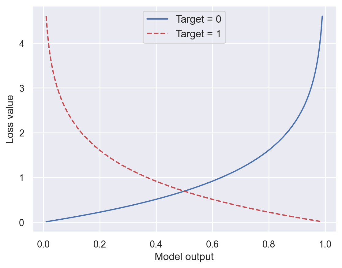
This choice depends on the problem type. For binary classification tasks where expected results are either 1 (True) or 0 (False), a popular choice is the Binary Cross Entropy loss, a.k.a. log(istic regression) loss. It is implemented in the scikit-learn log_loss function.
\(y^{(i)} \in \{0,1\}\): expected result for the \(i\)th sample.
\(y'^{(i)} = h_{\pmb{\omega}}(\pmb{x}^{(i)}) \in [0,1]\): model output for the \(i\)th sample, i.e. probability that the \(i\)th sample belongs to the positive class.
def plot_bce():
    """Plot BCE loss for one output"""

    x = np.linspace(0.01, 0.99, 200)
    plt.plot(x, -np.log(1 - x), label="Target = 0")
    plt.plot(x, -np.log(x), "r--", label="Target = 1")
    plt.xlabel("Model output")
    plt.ylabel("Loss value")
    plt.legend(fontsize=12)
    plt.show()
plot_bce()
# Compute BCE losses for pseudo-predictions

y_true = [0, 0, 1, 1]

# Good prediction
y_pred = [0.1, 0.2, 0.7, 0.99]
bce = log_loss(y_true, y_pred)
print(f"BCE loss (good prediction): {bce:.05f}")

# Compare theorical and computed values
np.testing.assert_almost_equal(
    -(np.log(0.9) + np.log(0.8) + np.log(0.7) + np.log(0.99)) / 4, bce, decimal=5
)

# Perfect prediction
y_pred = [0.0, 0.0, 1.0, 1.0]
print(f"BCE loss (perfect prediction): {log_loss(y_true, y_pred):.05f}")

# Awful prediction
y_pred = [0.9, 0.85, 0.17, 0.05]
print(f"BCE loss (awful prediction): {log_loss(y_true, y_pred):.05f}")
BCE loss (good prediction): 0.17381
BCE loss (perfect prediction): 0.00000
BCE loss (awful prediction): 2.24185
Training a binary classifier#
# Create a classifier using stochastic gradient descent and logistic loss
sgd_model = SGDClassifier(loss="log_loss")

# Train the model on data
sgd_model.fit(x_train, y_train_5)
SGDClassifier(loss='log_loss')In a Jupyter environment, please rerun this cell to show the HTML representation or trust the notebook.
On GitHub, the HTML representation is unable to render, please try loading this page with nbviewer.org.
SGDClassifier(loss='log_loss')
Assesing performance#
Thresholding model output#
A ML model computes probabilities (or scores that are transformed into probabilities). These decimal values are thresholded into discrete values to form the model’s prediction.
# Check model predictions for the first 10 training samples

samples = x_train[:10]

# Print binary predictions ("is the digit a 5 or not?")
print(sgd_model.predict(samples))

# Print prediction probabilities
sgd_model.predict_proba(samples).round(decimals=3)
[False False False False False False True False False False]
array([[1.   , 0.   ],
       [0.975, 0.025],
       [1.   , 0.   ],
       [1.   , 0.   ],
       [1.   , 0.   ],
       [0.993, 0.007],
       [0.172, 0.828],
       [1.   , 0.   ],
       [1.   , 0.   ],
       [1.   , 0.   ]])
Accuracy#
The default performance metric for classification taks is accuracy.
# Define fictitious ground truth and prediction results
y_true = np.array([1, 0, 0, 1, 1, 1])
y_pred = np.array([1, 1, 0, 1, 0, 1])

# Compute accuracy: 4/6 = 2/3
acc = np.sum(y_pred == y_true) / len(y_true)
print(f"{acc:.2f}")
0.67
Computing training accuracy#
# The score function computes accuracy of the SGDClassifier
train_acc = sgd_model.score(x_train, y_train_5)
print(f"Training accuracy: {train_acc:.05f}")

# Using cross-validation to better evaluate accuracy, using 3 folds
cv_acc = cross_val_score(sgd_model, x_train, y_train_5, cv=3, scoring="accuracy")
print(f"Cross-validation accuracy: {cv_acc}")
Training accuracy: 0.97212
Cross-validation accuracy: [0.96745 0.9737  0.97205]
Accuracy shortcomings#
When the dataset is skewed (some classes are more frequent than others), computing accuracy is not enough to assert the model’s performance.
To find out why, let’s imagine a dumb binary classifier that always predicts that the digit is not 5.
# Count the number of non-5 digits in the dataset
not5_count = len(y_train_5) - np.sum(y_train_5)
print(f"There are {not5_count} digits other than 5 in the training set")

dumb_model_acc = not5_count / len(x_train)
print(f"Dumb classifier accuracy: {dumb_model_acc:.05f}")
There are 54578 digits other than 5 in the training set
Dumb classifier accuracy: 0.90963
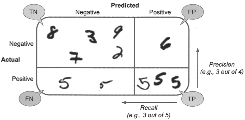
True/False positives and negatives#
True Positive (TP): the model correctly predicts the positive class.
False Positive (FP): the model incorrectly predicts the positive class.
True Negative (TN): the model correctly predicts the negative class.
False Negative (FN): the model incorrectly predicts the negative class.
Confusion matrix#
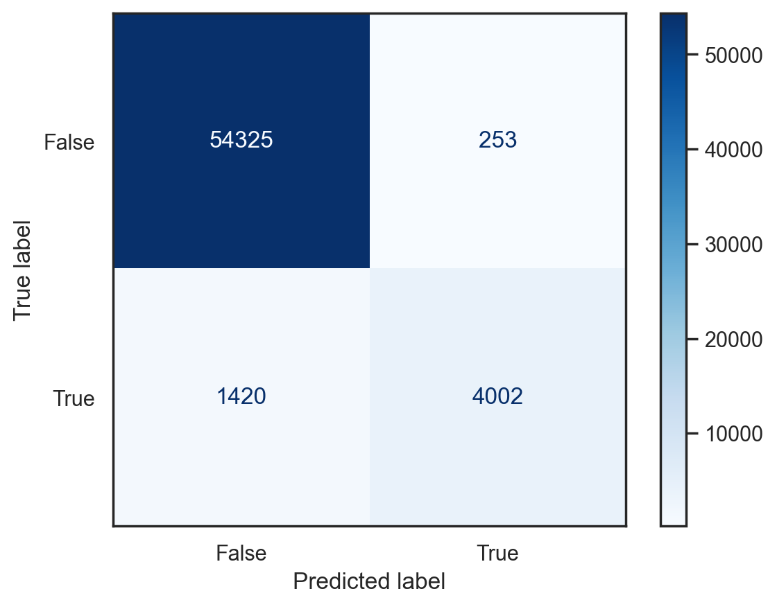
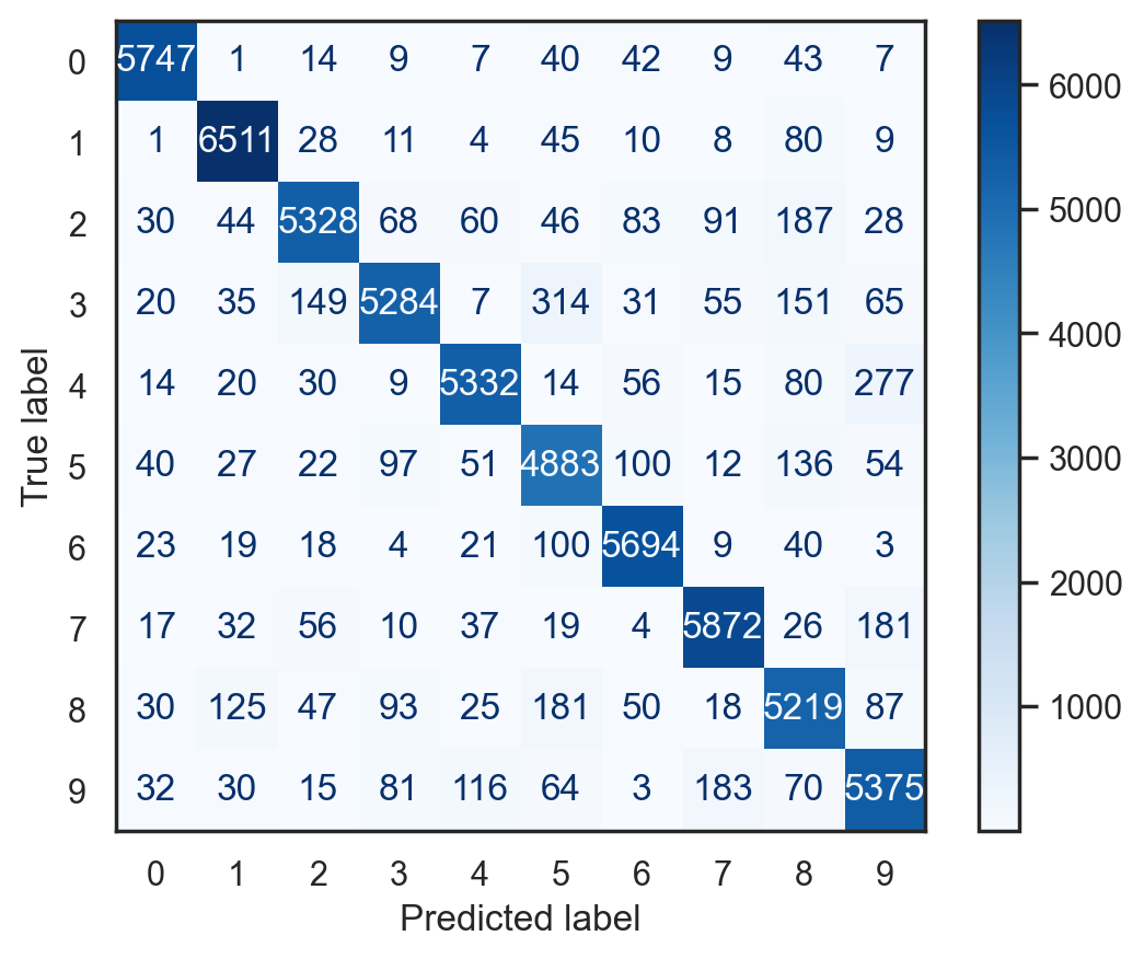
Useful representation of classification results. Row are actual classes, columns are predicted classes.
def plot_conf_mat(model, x, y):
    """Plot the confusion matrix for a model, inputs and targets"""

    with sns.axes_style("white"):  # Temporary hide Seaborn grid lines
        _ = ConfusionMatrixDisplay.from_estimator(
            model, x, y, values_format="d", cmap=plt.colormaps.get_cmap("Blues")
        )


# Plot confusion matrix for the SGDClassifier
plot_conf_mat(sgd_model, x_train, y_train_5)
Precision and recall#
Precision: proportion of all predictions for a class that were actually correct.
Recall: proportion of all samples for a class that were correctly predicted.
Example: for the positive class,
# Define fictitious ground truth and prediction results
y_true = np.array([1, 0, 0, 1, 1, 1])
y_pred = np.array([1, 1, 0, 1, 0, 0])

# Compute precision and recall for both classes
for label in [0, 1]:
    TP = np.sum((y_pred == label) & (y_true == label))
    FP = np.sum((y_pred == label) & (y_true == 1 - label))
    FN = np.sum((y_pred == 1 - label) & (y_true == label))
    print(f"Class {label}: Precision {TP/(TP+FP):.02f}, Recall {TP/(TP+FN):.02f}")
Class 0: Precision 0.33, Recall 0.50
Class 1: Precision 0.67, Recall 0.50
Example: a (flawed) tumor classifier#
Context: binary classification of tumors (positive means malignant). Dataset of 100 tumors, of which 9 are malignant.
Negatives |
Positives |
|---|---|
True Negatives: 90 |
False Positives: 1 |
False Negatives: 8 |
True Positives: 1 |
The precision/recall trade-off#
Improving precision typically reduces recall and vice versa (example).
Precision matters most when the cost of false positives is high (example: spam detection).
Recall matters most when the cost of false negatives is high (example: tumor detection).
F1 score#
Weighted average (harmonic mean) of precision and recall.
Also known as balanced F-score or F-measure.
Favors classifiers that have similar precision and recall.
# Compute several metrics about our 5/not 5 classifier
print(classification_report(y_train_5, sgd_model.predict(x_train)))
              precision    recall  f1-score   support

       False       0.97      1.00      0.98     54578
        True       0.94      0.74      0.83      5422

    accuracy                           0.97     60000
   macro avg       0.96      0.87      0.91     60000
weighted avg       0.97      0.97      0.97     60000
Multiclass classification#
Choosing a loss function#
The log loss extends naturally to the multiclass case. It is also called Negative Log-Likelihood or Cross Entropy, and is also implemented in the scikit-learn log_loss function.
\(\pmb{y^{(i)}} \in \{0,1\}^K\): binary vector of \(K\) elements.
\(y^{(i)}_k \in \{0,1\}\): expected value for the \(k\)th label of the \(i\)th sample. \(y^{(i)}_k = 1\) iff the \(i\)th sample has label \(k \in [1,K]\).
\(y'^{(i)}_k \in [0,1]\): model output for the \(k\)th label of the \(i\)th sample, i.e. probability that the \(i\)th sample has label \(k\).
# Compute cross entropy losses for pseudo-predictions

# 2 samples with 3 possibles labels. Sample 1 has label 2, sample 2 has label 3
y_true = [[0, 1, 0], [0, 0, 1]]

# Probability distribution vector
# 95% proba that sample 1 has label 2, 70% proba that sample 2 has label 3
y_pred = [[0.05, 0.95, 0], [0.1, 0.2, 0.7]]

# Compute cross entropy loss
ce = log_loss(y_true, y_pred)
print(f"Cross entropy loss: {ce:.05f}")

# Compare theorical and computed loss values
np.testing.assert_almost_equal(-(np.log(0.95) + np.log(0.7)) / 2, ce)
Cross entropy loss: 0.20398
Training a multiclass classifier#
# Using all digits as training results
y_train = train_targets
y_test = test_targets

# Training another SGD classifier to recognize all digits
multi_sgd_model = SGDClassifier(loss="log_loss")
multi_sgd_model.fit(x_train, y_train)
SGDClassifier(loss='log_loss')In a Jupyter environment, please rerun this cell to show the HTML representation or trust the notebook.
On GitHub, the HTML representation is unable to render, please try loading this page with nbviewer.org.
SGDClassifier(loss='log_loss')
Assessing performance#
# Since dataset is not class imbalanced anymore, accuracy is now a reliable metric
print(f"Training accuracy: {multi_sgd_model.score(x_train, y_train):.05f}")
print(f"Test accuracy: {multi_sgd_model.score(x_test, y_test):.05f}")
Training accuracy: 0.92075
Test accuracy: 0.91780
# Plot confusion matrix for the multiclass SGD classifier
plot_conf_mat(multi_sgd_model, x_train, y_train)
# Compute performance metrics about the multiclass SGD classifier
print(classification_report(y_train, multi_sgd_model.predict(x_train)))
              precision    recall  f1-score   support

           0       0.97      0.97      0.97      5919
           1       0.95      0.97      0.96      6707
           2       0.93      0.89      0.91      5965
           3       0.93      0.86      0.90      6111
           4       0.94      0.91      0.93      5847
           5       0.86      0.90      0.88      5422
           6       0.94      0.96      0.95      5931
           7       0.94      0.94      0.94      6254
           8       0.87      0.89      0.88      5875
           9       0.88      0.90      0.89      5969

    accuracy                           0.92     60000
   macro avg       0.92      0.92      0.92     60000
weighted avg       0.92      0.92      0.92     60000


