Data manipulation

Learning objectives

• Discover what tensors are and how to manipulate them with NumPy and PyTorch.

• Be able to load and prepare datasets of different types (tabular data, images or videos) for training a Machine Learning model.

• Learn how the pandas and scikit-learn libraries can help achieve the previous task.

Environment setup

# pylint: disable=wrong-import-position

import os

# Installing the ainotes package is only necessary in standalone runtime environments like Colab
if os.getenv("COLAB_RELEASE_TAG"):
    print("Standalone runtime environment detected, installing ainotes package")
    %pip install ainotes

# pylint: enable=wrong-import-position

import platform

import numpy as np
import matplotlib.pyplot as plt
import pandas as pd

import sklearn
from sklearn.datasets import load_sample_images
from sklearn.model_selection import train_test_split
from sklearn.impute import SimpleImputer
from sklearn.preprocessing import MinMaxScaler, StandardScaler, OneHotEncoder

import torch

from ainotes.utils.train import get_device

# Setup plots

# Include matplotlib graphs into the notebook, next to the code
# https://stackoverflow.com/a/43028034/2380880
%matplotlib inline

# Improve plot quality
%config InlineBackend.figure_format = "retina"

# Print environment info
print(f"Python version: {platform.python_version()}")
print(f"NumPy version: {np.__version__}")
print(f"scikit-learn version: {sklearn.__version__}")
print(f"PyTorch version: {torch.__version__}")


# PyTorch device configuration
device, message = get_device()
print(message)

Python version: 3.11.1
NumPy version: 1.26.4
scikit-learn version: 1.4.1.post1
PyTorch version: 2.2.1
Using MPS GPU :)

Working with tensors

Definition

In the context of AI, a tensor is a set of primitive values sharing the same type (most often numerical), shaped into an array of any number of dimensions. It is a fancy name for a multidimensional array.

Tensors are heavily used by AI algorithms to represent and manipulate information. They are, in particular, the core data structures of Machine Learning.

Tensor properties

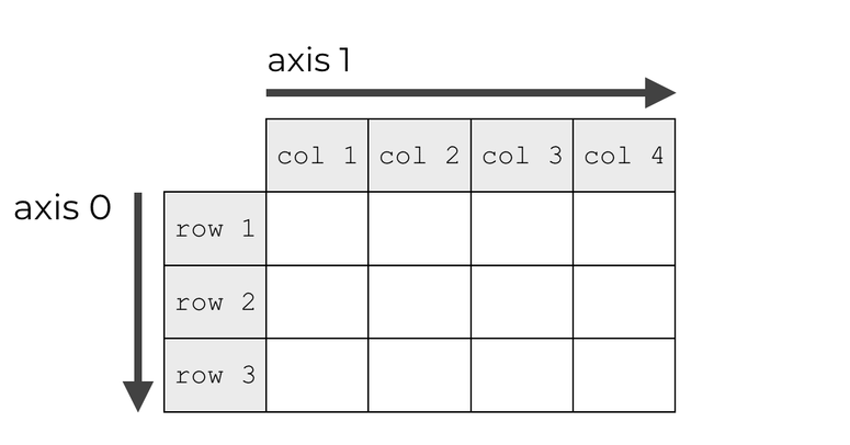
• A tensor’s dimension is also called an axis.

• A tensor’s rank is its number of axes.

• The tensor’s shape describes the number of values along each axis.

In mathematical terms, a rank 0 tensor is a scalar, a rank 1 tensor is a vector and a rank 2 tensor is a matrix.

Warning: rank and dimension are polysemic terms, which can be confusing.

Tensors in Python

Python offers limited native support for manipulating tensors. Lists can be used to store information, but their mathematical capacities are insufficient for any serious work.

# A vector (rank 1 tensor)
a = [1, 2, 3]
print(a)

# A matrix (rank 2 tensor)
b = [a, [4, 5, 6]]
print(b)

[1, 2, 3]
[[1, 2, 3], [4, 5, 6]]

Dedicated libraries

Over the years, several tools have been developed to overcome Python’s native limitations.

The most widely used is NumPy, which supports tensors in the form of ndarray objects. It offers a comprehensive set of operations on them, including creating, sorting, selecting, linear algebra and statistical operations.

Tensor management with NumPy

Creating tensors

The np.array function creates and returns a new tensor.

The NumPy API contains many functions for creating tensors using predefined values.

def print_tensor_info(t):
    """Print values, number of dimensions and shape of a tensor"""

    print(t)
    print(f"Dimensions: {t.ndim}")
    print(f"Shape: {t.shape}")

# Create a scalar
x = np.array(12)

print_tensor_info(x)

12
Dimensions: 0
Shape: ()

# Create a vector (1D tensor)
x = np.array([1, 2, 3])

print_tensor_info(x)

[1 2 3]
Dimensions: 1
Shape: (3,)

Generating random tensors

The NumPy API also permits the creation of (pseudo-)randomly valued tensors, using various statistical laws and data types.

# Init a NumPy random number generator
rng = np.random.default_rng()

# Create a 3x4 random matrix (2D tensor) with real values sampled from a uniform distribution
x = rng.uniform(size=(3, 4))

print_tensor_info(x)

[[0.87327715 0.69783603 0.91380947 0.95877851]
 [0.3600699  0.87642275 0.40869857 0.43925051]
 [0.54297924 0.77137579 0.81503553 0.34392423]]
Dimensions: 2
Shape: (3, 4)

# Create a 3x2x5 3D tensor with integer values sampled from a uniform distribution
x = rng.integers(low=0, high=100, size=(3, 2, 5))

print_tensor_info(x)

[[[97 16 21 94  2]
  [66 48 96  7 51]]

 [[10 32 50 31 30]
  [98 72 28  2 29]]

 [[11  7 20 85 10]
  [80 97 64 92 11]]]
Dimensions: 3
Shape: (3, 2, 5)

Shape management

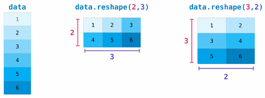
A common operation on tensors is reshaping: giving it a new shape without changing its data.

The new shape must be compatible with the current one: the new tensor needs to have the same number of elements as the original one.

# Reshape a 3x2 matrix into a 2x3 matrix
x = np.array([[1, 2], [3, 4], [5, 6]])
x_reshaped = x.reshape(2, 3)

print_tensor_info(x_reshaped)

[[1 2 3]
 [4 5 6]]
Dimensions: 2
Shape: (2, 3)

# Reshape the previous matrix into a vector
x_reshaped = x.reshape(
    6,
)

print_tensor_info(x_reshaped)

[1 2 3 4 5 6]
Dimensions: 1
Shape: (6,)

# Error: incompatible shapes!
# x.reshape(5, )

Indexing and slicing

Tensors can be indexed and sliced just like regular Python lists.

x = np.array([1, 2, 3])

# Select element at index 1
assert x[1] == 2

# Select elements between indexes 0 (included) and 2 (excluded)
assert np.array_equal(x[0:2], [1, 2])

# Select elements starting at index 1 (included)
assert np.array_equal(x[1:], [2, 3])

# Select last element
assert np.array_equal(x[-1], 3)

# Select all elements but last one
assert np.array_equal(x[:-1], [1, 2])

# Select last 2 elements
assert np.array_equal(x[-2:], [2, 3])

# Select second-to-last element
assert np.array_equal(x[-2:-1], [2])

Tensor axes

Many tensor operations can be applied along one or several axes. They are indexed starting at 0.

# Create a 2x2 matrix (2D tensor)
x = np.array([[1, 1], [2, 2]])
print(x)

# Summing values on first axis (rows)
print(x.sum(axis=0))

# Summing values on second axis (columns)
print(x.sum(axis=1))

[[1 1]
 [2 2]]
[3 3]
[2 4]

Element-wise operations

These operations are applied independently to each entry in the tensors being considered.

# Element-wise product between two matrices (shapes must be identical)
x = np.array([[1, 2, 3], [3, 2, -2]])
y = np.array([[3, 0, 2], [1, 4, -2]])
z = x * y

print(x)
print(y)
print_tensor_info(z)

[[ 1  2  3]
 [ 3  2 -2]]
[[ 3  0  2]
 [ 1  4 -2]]
[[3 0 6]
 [3 8 4]]
Dimensions: 2
Shape: (2, 3)

Dot product

On the contrary, operations like dot product combine entries in the input tensors to produce a differently shaped result.

# Dot product between two matrices (shapes must be compatible)
x = np.array([[1, 2, 3], [3, 2, 1]])
y = np.array([[3, 0], [2, 1], [4, -2]])
# alternative syntax: z = x.dot(y)
z = np.dot(x, y)

print(x)
print(y)
print_tensor_info(z)

[[1 2 3]
 [3 2 1]]
[[ 3  0]
 [ 2  1]
 [ 4 -2]]
[[19 -4]
 [17  0]]
Dimensions: 2
Shape: (2, 2)

Broadcasting

Broadcasting is a mechanism that allows operations to be performed on tensors of different shapes. Subject to certain constraints, the smaller tensor may be “broadcast” across the larger one so that they have compatible shapes.

Broadcasting provides a efficient means of vectorizing tensor operations.

# Broadcasting between a vector and a scalar
x = np.array([1.0, 2.0])
print(x * 1.6)

[1.6 3.2]

# Broadcasting between a matrix and a vector
x = np.array([[0, 1, 2], [-2, 5, 3]])
y = np.array([1, 2, 3])
z = x + y

print_tensor_info(z)

[[ 1  3  5]
 [-1  7  6]]
Dimensions: 2
Shape: (2, 3)

GPU-based tensors

For all its qualities, NumPy has a limitation which can be critical in some contexts: it only runs on the machine’s CPU.

Among other advantages, newer tools offer support for dedicated high-performance processors like GPUs or TPUs, while providing a NumPy-like API to make onboarding easier. The most prominent ones are currently TensorFlow, PyTorch and JAX.

# Create a 2x2 random PyTorch tensor, trying to store it into the GPU memory
x = torch.rand(size=(2, 2), device=device)
print(x)

tensor([[0.5224, 0.7456],
        [0.5272, 0.0403]], device='mps:0')

/Users/baptiste/Documents/Projets/GitHub/bpesquet/ainotes/.venv/lib/python3.11/site-packages/torch/_tensor_str.py:137: UserWarning: MPS: nonzero op is supported natively starting from macOS 13.0. Falling back on CPU. This may have performance implications. (Triggered internally at /Users/runner/work/pytorch/pytorch/pytorch/aten/src/ATen/native/mps/operations/Indexing.mm:283.)
  nonzero_finite_vals = torch.masked_select(

Loading and exploring data

Introduction to pandas

The pandas library is dedicated to data analysis in Python. It greatly facilitates loading, exploring and processing tabular data files.

The primary data structures in pandas are implemented as two classes:

• DataFrame, which is quite similar to as a relational data table, with rows and named columns.

• Series, which represents a single data column. A DataFrame contains one or more Series and a name for each Series.

The DataFrame is a commonly used abstraction for data manipulation.

# Create two data Series
pop = pd.Series({"CAL": 38332521, "TEX": 26448193, "NY": 19651127})
area = pd.Series({"CAL": 423967, "TEX": 695662, "NY": 141297})

# Create a DataFrame contraining the two Series
# The df_ prefix is used to distinguish pandas dataframes from plain NumPy arrays
df_poprep = pd.DataFrame({"population": pop, "area": area})

print(df_poprep)

     population    area
CAL    38332521  423967
TEX    26448193  695662
NY     19651127  141297

Loading a tabular dataset

When describing tabular information, most datasets are stored as a CSV (Comma-Separated Values) text file.

The pd.read_csv function can load a CSV file into a DataFrame from either a local path or a URL.

The following code loads a dataset which was extracted from a Kaggle competition.

# Load a CSV file into a DataFrame
# Data comes from this Kaggle competition:
df_olympics = pd.read_csv(
    "https://raw.githubusercontent.com/bpesquet/ainotes/master/data/athlete_events.csv"
)

Exploring tabular data

Once a dataset is loaded into a DataFrame, many operations can be applied to it for visualization or transformation purposes. For more details, see the 10 minutes to pandas tutorial.

Let’s use pandas to perform the very first steps of what is often called Exploratory Data Analysis.

# Print dataset shape (rows x columns)
print(f"df_olympics: {df_olympics.shape}")

df_olympics: (271116, 15)

# Print a concise summary of the dataset
df_olympics.info()

<class 'pandas.core.frame.DataFrame'>
RangeIndex: 271116 entries, 0 to 271115
Data columns (total 15 columns):
 #   Column  Non-Null Count   Dtype  
---  ------  --------------   -----  
 0   ID      271116 non-null  int64  
 1   Name    271116 non-null  object 
 2   Sex     271116 non-null  object 
 3   Age     261642 non-null  float64
 4   Height  210945 non-null  float64
 5   Weight  208241 non-null  float64
 6   Team    271116 non-null  object 
 7   NOC     271116 non-null  object 
 8   Games   271116 non-null  object 
 9   Year    271116 non-null  int64  
 10  Season  271116 non-null  object 
 11  City    271116 non-null  object 
 12  Sport   271116 non-null  object 
 13  Event   271116 non-null  object 
 14  Medal   39783 non-null   object 
dtypes: float64(3), int64(2), object(10)
memory usage: 31.0+ MB

# Print the first 10 rows of the dataset
df_olympics.head(n=10)

	ID	Name	Sex	Age	Height	Weight	Team	NOC	Games	Year	Season	City	Sport	Event	Medal
0	1	A Dijiang	M	24.0	180.0	80.0	China	CHN	1992 Summer	1992	Summer	Barcelona	Basketball	Basketball Men's Basketball	NaN
1	2	A Lamusi	M	23.0	170.0	60.0	China	CHN	2012 Summer	2012	Summer	London	Judo	Judo Men's Extra-Lightweight	NaN
2	3	Gunnar Nielsen Aaby	M	24.0	NaN	NaN	Denmark	DEN	1920 Summer	1920	Summer	Antwerpen	Football	Football Men's Football	NaN
3	4	Edgar Lindenau Aabye	M	34.0	NaN	NaN	Denmark/Sweden	DEN	1900 Summer	1900	Summer	Paris	Tug-Of-War	Tug-Of-War Men's Tug-Of-War	Gold
4	5	Christine Jacoba Aaftink	F	21.0	185.0	82.0	Netherlands	NED	1988 Winter	1988	Winter	Calgary	Speed Skating	Speed Skating Women's 500 metres	NaN
5	5	Christine Jacoba Aaftink	F	21.0	185.0	82.0	Netherlands	NED	1988 Winter	1988	Winter	Calgary	Speed Skating	Speed Skating Women's 1,000 metres	NaN
6	5	Christine Jacoba Aaftink	F	25.0	185.0	82.0	Netherlands	NED	1992 Winter	1992	Winter	Albertville	Speed Skating	Speed Skating Women's 500 metres	NaN
7	5	Christine Jacoba Aaftink	F	25.0	185.0	82.0	Netherlands	NED	1992 Winter	1992	Winter	Albertville	Speed Skating	Speed Skating Women's 1,000 metres	NaN
8	5	Christine Jacoba Aaftink	F	27.0	185.0	82.0	Netherlands	NED	1994 Winter	1994	Winter	Lillehammer	Speed Skating	Speed Skating Women's 500 metres	NaN
9	5	Christine Jacoba Aaftink	F	27.0	185.0	82.0	Netherlands	NED	1994 Winter	1994	Winter	Lillehammer	Speed Skating	Speed Skating Women's 1,000 metres	NaN

# Print 5 random samples
df_olympics.sample(n=5)

	ID	Name	Sex	Age	Height	Weight	Team	NOC	Games	Year	Season	City	Sport	Event	Medal
234619	117659	Andrzej Szymczak	M	27.0	193.0	96.0	Poland	POL	1976 Summer	1976	Summer	Montreal	Handball	Handball Men's Handball	Bronze
165291	83006	John William Mulhall	M	26.0	165.0	62.0	Great Britain	GBR	1964 Summer	1964	Summer	Tokyo	Gymnastics	Gymnastics Men's Horse Vault	NaN
226761	113946	Barbora potkov	F	31.0	182.0	80.0	Czech Republic	CZE	2012 Summer	2012	Summer	London	Athletics	Athletics Women's Javelin Throw	Gold
223951	112493	Clement Eyer Smoot	M	20.0	NaN	NaN	Western Golf Association-1	USA	1904 Summer	1904	Summer	St. Louis	Golf	Golf Men's Team	Gold
196758	98783	Shankar Ramu	M	22.0	NaN	NaN	Malaysia	MAS	1992 Summer	1992	Summer	Barcelona	Hockey	Hockey Men's Hockey	NaN

# Print descriptive statistics for all numerical attributes
df_olympics.describe()

	ID	Age	Height	Weight	Year
count	271116.000000	261642.000000	210945.000000	208241.000000	271116.000000
mean	68248.954396	25.556898	175.338970	70.702393	1978.378480
std	39022.286345	6.393561	10.518462	14.348020	29.877632
min	1.000000	10.000000	127.000000	25.000000	1896.000000
25%	34643.000000	21.000000	168.000000	60.000000	1960.000000
50%	68205.000000	24.000000	175.000000	70.000000	1988.000000
75%	102097.250000	28.000000	183.000000	79.000000	2002.000000
max	135571.000000	97.000000	226.000000	214.000000	2016.000000

# Print descriptive statistics for all non-numerical attributes
df_olympics.describe(include=["object", "bool"])

	Name	Sex	Team	NOC	Games	Season	City	Sport	Event	Medal
count	271116	271116	271116	271116	271116	271116	271116	271116	271116	39783
unique	134732	2	1184	230	51	2	42	66	765	3
top	Robert Tait McKenzie	M	United States	USA	2000 Summer	Summer	London	Athletics	Football Men's Football	Gold
freq	58	196594	17847	18853	13821	222552	22426	38624	5733	13372

# Print the number of samples by sport
df_olympics["Sport"].value_counts()

Sport
Athletics        38624
Gymnastics       26707
Swimming         23195
Shooting         11448
Cycling          10859
                 ...  
Racquets            12
Jeu De Paume        11
Roque                4
Basque Pelota        2
Aeronautics          1
Name: count, Length: 66, dtype: int64

# Print rounded average age for women
age_mean = df_olympics[df_olympics["Sex"] == "F"]["Age"].mean()
print(f"{age_mean:.0f}")

24

# Print percent of athletes for some countries

athletes_count = df_olympics.shape[0]

for country in ["USA", "FRA", "GBR", "GER"]:
    percent = (df_olympics["NOC"] == country).sum() / athletes_count
    print(f"Athletes from {country}: {percent*100:.2f}%")

Athletes from USA: 6.95%
Athletes from FRA: 4.71%
Athletes from GBR: 4.52%
Athletes from GER: 3.63%

Loading images

Digital images are stored using either the bitmap format (an array of color values for all individual pixels in the image) or the vector format (a description of the elementary shapes in the image).

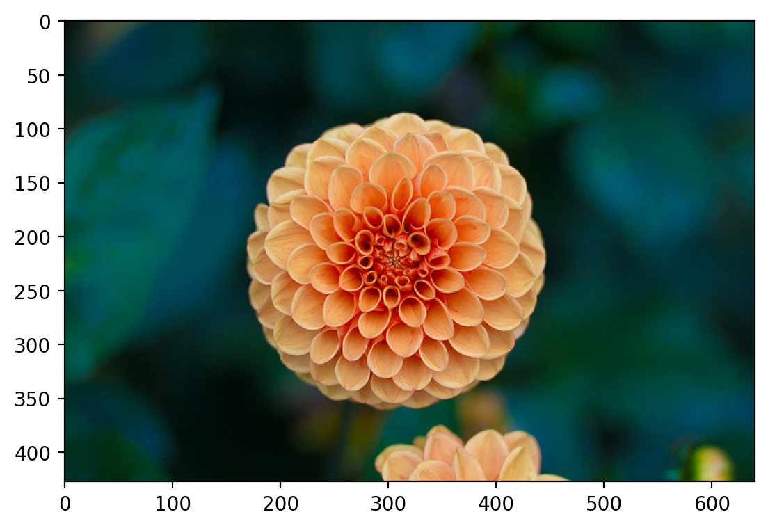
Bitmap images can be easily manipulated as tensors. Each pixel color is typically expressed using a combination of the three primary colors: red, green and blue.

# Load sample images provided by scikit-learn into a NumPy array
images = np.asarray(load_sample_images().images)

# Load the last sample image
sample_image = images[-1]

# Show image
plt.imshow(sample_image)

print(f"Images: {images.shape}")
print(f"Sample image: {sample_image.shape}")
print(f"Sample pixel: {sample_image[225, 300]}")

Images: (2, 427, 640, 3)
Sample image: (427, 640, 3)
Sample pixel: [219  78  60]

Preparing data for training

A mandatory step

In Machine Learning, the chosen dataset has to be carefully prepared before using it to train a model. This can have a major impact on the outcome of the training process.

This important task, sometimes called data preprocessing, might involve:

• Splitting data between training, validation and test sets.

• Reshaping data.

• Removing superflous features (if any).

• Adding missing values.

• Scaling data.

• Transforming values into numeric form.

• Augmenting data.

• Engineering new features.

Data splitting

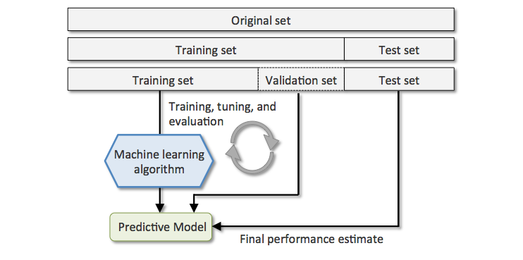
Once trained, a ML model must be able to generalize (perform well with new data). In order to assert this ability, data is always split into two or three sets before training:

• Training set (typically 80% or more): fed to the model during training.

• Validation set: used to tune the model without biasing it in favor of the test set.

• Test set: used to check the final model’s performance on unseen data.

# Demonstrate the use of scikit-learn's train_test_split for splitting a dataset

# Create a random 30x4 matrix (fictitious inputs) and a random 30x1 vector (fictitious results)
x = np.random.rand(30, 4)
y = np.random.rand(30)
print(f"x: {x.shape}. y: {y.shape}")

# Split fictitious dataset between training and test sets, using a 75/25 ratio
# A unique call to train_test_split is mandatory to maintain inputs/target correspondance between samples
# https://scikit-learn.org/stable/modules/generated/sklearn.model_selection.train_test_split.html
x_train, x_test, y_train, y_test = train_test_split(x, y, test_size=0.25)

print(f"x_train: {x_train.shape}. y_train: {y_train.shape}")
print(f"x_test: {x_test.shape}. y_test: {y_test.shape}")

x: (30, 4). y: (30,)
x_train: (22, 4). y_train: (22,)
x_test: (8, 4). y_test: (8,)

Image and video reshaping

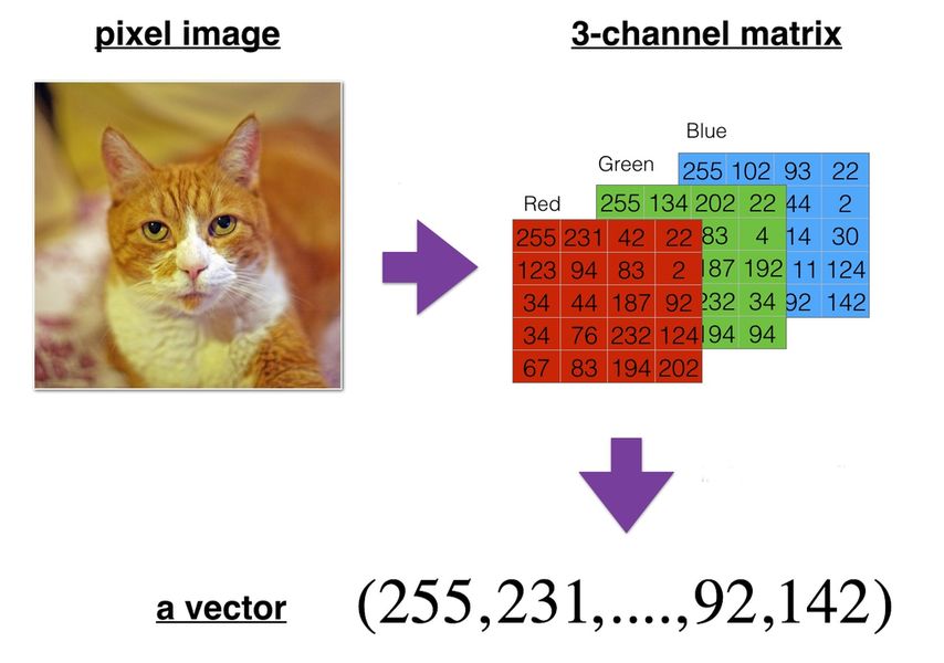
A bitmap image can be represented as a 3D multidimensional array of dimensions \(height \times width \times color\_channels\).

A video can be represented as a 4D multidimensional array of dimensions \(frames \times height \times width \times color\_channels\).

They have to be reshaped, or more precisely flattened in that case, into a vector (1D tensor) before being fed to most ML algorithms.

# Flatten the image, which is a 3D tensor, into a vector (1D tensor)
flattened_image = sample_image.reshape((427 * 640 * 3,))

# Alternative syntaxes to achieve the same result
# -1 means the new dimension is inferred from current dimensions
# Diference between flatten() and ravel() is explained here:
# https://numpy.org/doc/stable/user/absolute_beginners.html#reshaping-and-flattening-multidimensional-arrays
flattened_image = sample_image.reshape((-1,))
flattened_image = sample_image.ravel()
flattened_image = sample_image.flatten()

print(f"Flattened image: {flattened_image.shape}")

Flattened image: (819840,)

Handling of missing values

Most ML algorithms cannot work with missing values in features.

Depending on the percentage of missing data, three options exist:

• remove the corresponding data samples;

• remove the whole feature(s);

• replace the missing values (using 0, the mean, the median or something more meaningful in the context).

# Demonstrate the use of scikit-learn's SimpleImputer for handling missing values

# Create a tensor with missing values
x = np.array([[7, 2, np.nan], [4, np.nan, 6], [10, 5, 9]])
print(x)

# Replace missing values with column-wise mean
imputer = SimpleImputer(strategy="mean")
print(imputer.fit_transform(x))

# Replace missing values with "Unknown"
imputer = SimpleImputer(strategy="constant", missing_values=None, fill_value="Unknown")
print(imputer.fit_transform([["M"], ["M"], [None], ["F"], [None]]))

[[ 7.  2. nan]
 [ 4. nan  6.]
 [10.  5.  9.]]
[[ 7.   2.   7.5]
 [ 4.   3.5  6. ]
 [10.   5.   9. ]]
[['M']
 ['M']
 ['Unknown']
 ['F']
 ['Unknown']]

Feature scaling

Most ML algorithms work best when all features have a similar scale. Several solutions exist:

• Min-Max scaling: features are shifted and rescaled to the \([0,1]\) range by substracting the min value and dividing by (max-min) on the first axis.

• Standardization: features are centered (substracted by their mean) then reduced (divided by their standard deviation) on the first axis. All resulting features have a mean of 0 and a standard deviation of 1.

# Demonstrate the use of scikit-learn's MinMaxScaler to rescale values

# Generate a random 3x4 tensor with integer values between 1 and 10
x = np.random.randint(1, 10, (3, 4))
print(x)

# Compute min and max then scale tensor in one operation
x_scaled = MinMaxScaler().fit_transform(x)

print(x_scaled)
print(f"Minimum: {x_scaled.min(axis=0)}. Maximum: {x_scaled.max(axis=0)}")

[[4 2 1 1]
 [4 9 7 4]
 [3 1 9 3]]
[[1.         0.125      0.         0.        ]
 [1.         1.         0.75       1.        ]
 [0.         0.         1.         0.66666667]]
Minimum: [0. 0. 0. 0.]. Maximum: [1. 1. 1. 1.]

# Demonstrate the use of scikit-learn's StandardScaler to standardize values

# Generate a random (3,4) tensor with integer values between 1 and 10
x = np.random.randint(1, 10, (3, 4))
print(x)

# Center and reduce data
scaler = StandardScaler().fit(x)
print(scaler.mean_)

x_scaled = scaler.transform(x)
print(x_scaled)

# New mean is 0. New standard deviation is 1
print(f"Mean: {x_scaled.mean()}. Std: {x_scaled.std()}")

[[8 3 6 7]
 [2 7 7 6]
 [7 9 8 5]]
[5.66666667 6.33333333 7.         6.        ]
[[ 0.88900089 -1.33630621 -1.22474487  1.22474487]
 [-1.3970014   0.26726124  0.          0.        ]
 [ 0.50800051  1.06904497  1.22474487 -1.22474487]]
Mean: 1.850371707708594e-17. Std: 1.0

Feature scaling and training/test sets

In order to avoid information leakage, the test set must be scaled with values calculated on the training set.

# Compute mean and std on training set
scaler = StandardScaler().fit(x_train)

# Standardize training and test sets, using mean and std computed on training set
x_train_scaled = scaler.transform(x_train)
x_test_scaled = scaler.transform(x_test)

print(f"Train mean: {x_train_scaled.mean(axis=0)}")
print(f"Train std: {x_train_scaled.std(axis=0)}")
print(f"Test mean: {x_test_scaled.mean(axis=0)}")
print(f"Test std: {x_test_scaled.std(axis=0)}")

Train mean: [ 1.71579922e-16 -1.36885452e-16 -6.92627773e-16 -2.52323415e-17]
Train std: [1. 1. 1. 1.]
Test mean: [ 0.38510838  0.74722209  0.15848908 -0.06560817]
Test std: [0.95896239 1.37968827 1.12558319 1.33617739]

Image and video scaling

Individual pixel values for images and videos are typically integers in the \([0,255]\) range. This is not ideal for most ML algorithms.

Dividing them by \(255.0\) to obtain floats into the \([0,1]\) range is a common practice.

# Scaling sample image pixels between 0 and 1
scaled_image = sample_image / 255.0

# Check that all values are in the [0,1] range
assert scaled_image.min() >= 0
assert scaled_image.max() <= 1

Encoding of categorical features

Some features or targets may come as discrete rather than continuous values. Moreover, these discrete values might be strings. ML models are only able to manage numerical-only data.

A solution is to apply one-of-K encoding, also named dummy encoding or one-hot encoding. Each categorical feature with K possible values is transformed into a vector of K binary features, with one of them 1 and all others 0.

Note: using arbitrary integer values rather than binary vectors would create a proximity relationship between the new features, which could confuse the model during training.

# Demonstrate the use of scikit-learn's OneHotEncoder to one-hot encode categorical features

# Create a categorical variable with 3 different values
x = [["GOOD"], ["AVERAGE"], ["GOOD"], ["POOR"], ["POOR"]]

# Encoder input must be a matrix
# Output will be a sparse matrix where each column corresponds to one possible value of one feature
encoder = OneHotEncoder().fit(x)
x_hot = encoder.transform(x).toarray()

print(x_hot)
print(encoder.categories_)

[[0. 1. 0.]
 [1. 0. 0.]
 [0. 1. 0.]
 [0. 0. 1.]
 [0. 0. 1.]]
[array(['AVERAGE', 'GOOD', 'POOR'], dtype=object)]

# Demonstrate one-hot encoding of categorical features given as integers

# Generate a (5,1) tensor with integer values between 0 and 9
x = np.random.randint(0, 9, (5, 1))
print(x)

# Encoder input must be a matrix
# Output will be a sparse matrix where each column corresponds to one possible value of one feature
x_hot = OneHotEncoder().fit_transform(x).toarray()

print(x_hot)

[[0]
 [2]
 [6]
 [6]
 [0]]
[[1. 0. 0.]
 [0. 1. 0.]
 [0. 0. 1.]
 [0. 0. 1.]
 [1. 0. 0.]]

One-hot encoding and training/test sets

Depending on value distribution between training and test sets, some categories might appear only in one set.

The best solution is to one-hot encode based on the training set categories, ignoring test-only categories.

x_train = [["Blue"], ["Red"], ["Blue"], ["Green"]]
# "Yellow" is not present in training set
x_test = [
    ["Red"],
    ["Yellow"],
    ["Green"],
    ["Yellow"],
]

# Using categories from train set, ignoring unkwown categories
encoder = OneHotEncoder(handle_unknown="ignore").fit(x_train)
print(encoder.transform(x_train).toarray())
print(encoder.categories_)

# Unknown categories will result in a binary vector will all zeros
print(encoder.transform(x_test).toarray())

[[1. 0. 0.]
 [0. 0. 1.]
 [1. 0. 0.]
 [0. 1. 0.]]
[array(['Blue', 'Green', 'Red'], dtype=object)]
[[0. 0. 1.]
 [0. 0. 0.]
 [0. 1. 0.]
 [0. 0. 0.]]

x = [["M"], ["M"], [None], ["F"]]

# Replace missing values with constant
print(
    SimpleImputer(
        strategy="constant", missing_values=None, fill_value="Unknown"
    ).fit_transform(x)
)

[['M']
 ['M']
 ['Unknown']
 ['F']]

Data augmentation

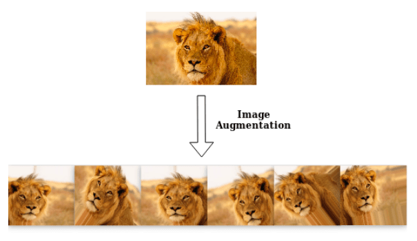
Data augmentation is the process of enriching a dataset by adding new samples, slightly modified copies of existing data or newly created synthetic data.

Feature engineering

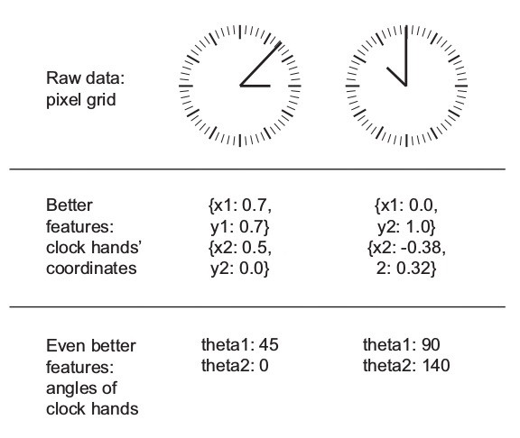
Feature engineering is the process of preparing the proper input features, in order to facilitate the learning task. The problem is made easier by expressing it in a simpler way. This usually requires a good domain knowledge.

The ability of deep neural networks to discover useful features by themselves has somewhat reduced the criticality of feature engineering. Nevertheless, it remains important in order to solve problems more elegantly and with fewer data.

Example (taken from the book Deep Learning with Python): the task of learning the time of day from a clock is far easier with engineered features rather than raw clock images.